[ acf , lags ] = autocorr( y ) returns the sample autocorrelation function (ACF) and associated lags of the input univariate time series.
ACFTbl = autocorr( Tbl ) returns a table containing variables for the sample ACF and associated lags of the last variable in the input table or timetable. To select a different variable for which to compute the ACF, use the DataVariable name-value argument. (since R2022a)
[ ___ , bounds ] = autocorr( ___ ) uses any input-argument combination in the previous syntaxes, and returns the output-argument combination for the corresponding input arguments and the approximate upper and lower confidence bounds on the ACF.
[ ___ ] = autocorr( ___ , Name=Value ) uses additional options specified by one or more name-value arguments. For example, autocorr(Tbl,DataVariable="RGDP",NumLags=10,NumSTD=1.96) returns 10 lags of the sample ACF of the table variable "RGDP" in Tbl and 95% confidence bounds.
autocorr( ___ ) plots the sample ACF of the input series with confidence bounds.
autocorr( ax , ___ ) plots on the axes specified by ax instead of the current axes ( gca ). ax can precede any of the input argument combinations in the previous syntaxes.
[ ___ , h ] = autocorr( ___ ) plots the sample ACF of the input series and additionally returns handles to plotted graphics objects. Use elements of h to modify properties of the plot after you create it.
Compute the ACF of a univariate time series. Input the time series data as a numeric vector.
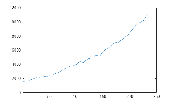
Load the quarterly real GDP series in Data_GDP.mat . Plot the series, which is stored in the numeric vector Data .
load Data_GDP plot(Data)
The series exhibits exponential growth.
Compute the returns of the series.
ret = price2ret(Data);
ret is a series of real GDP returns; it has one less observation than the real GDP series.
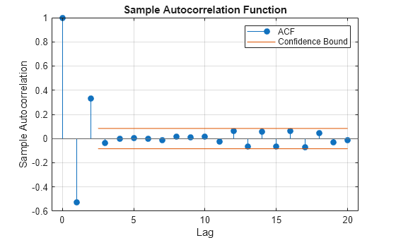
Compute the ACF of the real GDP returns, and return the associated lags.
[acf,lags] = autocorr(ret); [acf lags]
ans = 21×2 1.0000 0 0.3329 1.0000 0.1836 2.0000 -0.0216 3.0000 -0.1172 4.0000 -0.1632 5.0000 -0.0870 6.0000 -0.0707 7.0000 -0.0380 8.0000 0.0554 9.0000 ⋮
Let y t be the real GDP return at time t . In general, acf( j ) = Corr( y t , y t - lags ( j ) ). Therefore, acf(1) = Corr( y t , y t ) = 1.0000 , acf(2) = Corr( y t , y t - 1 ) = 0.3329 , and so on.
Compute the ACF of a time series, which is one variable in a table.
Load the electricity spot price data set Data_ElectricityPrices.mat , which contains the daily spot prices in the timetable DataTimeTable .
load Data_ElectricityPrices.mat DataTimeTable.Properties.VariableNames
ans = 1x1 cell array
Plot the series.
plot(DataTimeTable.SpotPrice)
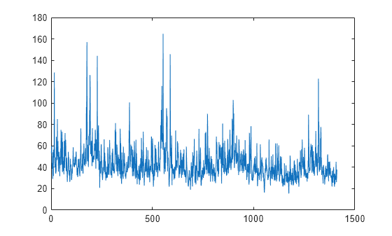
The time series plot does not clearly indicate an exponential trend or unit root.
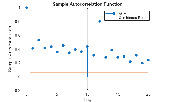
Compute the ACF of the raw spot price series.
ACFTbl = autocorr(DataTimeTable)
ACFTbl=21×2 table Lags ACF ____ _______ 0 1 1 0.55405 2 0.38251 3 0.31713 4 0.25107 5 0.21436 6 0.21275 7 0.19396 8 0.18292 9 0.18826 10 0.19476 11 0.19043 12 0.19963 13 0.19397 14 0.19957 15 0.25495 ⋮
autocorr returns the results in the table ACFTbl , where variables correspond to the ACF ( ACF ) and associated lags (Lags) .
By default, autocorr computes the ACF of the last variable in the table. To select a variable from an input table, set the DataVariable option.
Consider the electricity spot prices in Compute ACF of Table Variable.
Load the electricity spot price data set Data_ElectricityPrices.mat . Compute the ACF and return the ACF confidence bounds.
load Data_ElectricityPrices [ACFTbl,bounds] = autocorr(DataTimeTable)
ACFTbl=21×2 table Lags ACF ____ _______ 0 1 1 0.55405 2 0.38251 3 0.31713 4 0.25107 5 0.21436 6 0.21275 7 0.19396 8 0.18292 9 0.18826 10 0.19476 11 0.19043 12 0.19963 13 0.19397 14 0.19957 15 0.25495 ⋮
bounds = 2×1 0.0532 -0.0532
Assuming the spot prices follow a Gaussian white noise series, an approximate 95.4% confidence interval on the ACF is (-0.0532, 0.0532).
Although various estimates of the sample autocorrelation function exist, autocorr uses the form in Box, Jenkins, and Reinsel, 1994. In their estimate, they scale the correlation at each lag by the sample variance ( var(y,1) ) so that the autocorrelation at lag 0 is unity. However, certain applications require rescaling the normalized ACF by another factor.
Simulate 1000 observations from the standard Gaussian distribution.
rng(1); % For reproducibility y = randn(1000,1);
Compute the normalized and unnormalized sample ACF.
[normalizedACF, lags] = autocorr(y,NumLags=10); unnormalizedACF = normalizedACF*var(y,1);
Compare the first 10 lags of the sample ACF with and without normalization.
[lags normalizedACF unnormalizedACF]
ans = 11×3 0 1.0000 0.9960 1.0000 -0.0180 -0.0180 2.0000 0.0536 0.0534 3.0000 -0.0206 -0.0205 4.0000 -0.0300 -0.0299 5.0000 -0.0086 -0.0086 6.0000 -0.0108 -0.0107 7.0000 -0.0116 -0.0116 8.0000 0.0309 0.0307 9.0000 0.0341 0.0340 ⋮
Specify the MA(2) model:
y t = ε t - 0 . 5 ε t - 1 + 0 . 4 ε t - 2 ,
where ε t is Gaussian with mean 0 and variance 1.
rng(1); % For reproducibility Mdl = arima(MA=,Constant=0,Variance=1)
Mdl = arima with properties: Description: "ARIMA(0,0,2) Model (Gaussian Distribution)" SeriesName: "Y" Distribution: Name = "Gaussian" P: 0 D: 0 Q: 2 Constant: 0 AR: <> SAR: <> MA: at lags [1 2] SMA: <> Seasonality: 0 Beta: [1×0] Variance: 1
Simulate 1000 observations from Mdl .
y = simulate(Mdl,1000);
Plot the ACF of the simulated series. Specify that the series is an MA(2) process.
autocorr(y,NumMA=2)
The ACF cuts off after the second lag. This behavior is indicative of an MA(2) process.
Specify the multiplicative seasonal ARMA ( 2 , 0 , 1 ) × ( 3 , 0 , 0 ) 1 2 model:
( 1 - 0 . 7 5 L - 0 . 1 5 L 2 ) ( 1 - 0 . 9 L 1 2 + 0 . 5 L 2 4 - 0 . 5 L 3 6 ) y t = 2 + ε t - 0 . 5 ε t - 1 ,
where ε t is Gaussian with mean 0 and variance 1.
Mdl = arima(AR=,SAR=, . SARLags=[12 24 36],MA=-0.5,Constant=2, . Variance=1);
Simulate data from Mdl .
rng(1); % For reproducibility y = simulate(Mdl,1000);
Plot the default autocorrelation function (ACF).
figure autocorr(y)
The default correlogram does not display the dependence structure for higher lags.
Plot the ACF for 40 lags.
figure autocorr(y,NumLags=40)
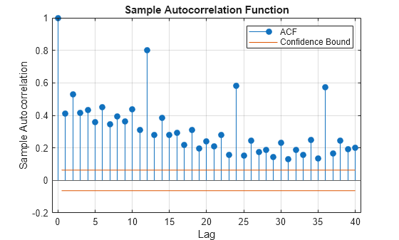
The correlogram shows the larger correlations at lags 12, 24, and 36.
Observed univariate time series for which autocorr computes or plots the ACF, specified as a numeric vector.
Data Types: double
Time series data, specified as a table or timetable. Each row of Tbl contains contemporaneous observations of all variables.
Specify a single series (variable) by using the DataVariable argument. The selected variable must be numeric.
Axes on which to plot, specified as an Axes object.
By default, autocorr plots to the current axes ( gca ).
Note
Specify missing observations using NaN . The autocorr function treats missing values as missing completely at random.
Specify optional pairs of arguments as Name1=Value1. NameN=ValueN , where Name is the argument name and Value is the corresponding value. Name-value arguments must appear after other arguments, but the order of the pairs does not matter.
Before R2021a, use commas to separate each name and value, and enclose Name in quotes.
Example: autocorr(Tbl,DataVariable="RGDP",NumLags=10,NumSTD=3) plots 10 lags of the sample ACF of the variable "RGDP" in Tbl , and displays confidence bounds consisting of 3 standard errors away from 0.
Number of lags in the sample ACF, specified as a positive integer. autocorr uses lags 0:NumLags to estimate the ACF.
The default is min([20, T – 1]) , where T is the effective sample size of the input time series.
Example: autocorr(y,NumLags=10) plots the sample ACF of y for lags 0 through 10 .
Data Types: double
Number of lags in a theoretical MA model of the input time series, specified as a nonnegative integer less than NumLags .
autocorr uses NumMA to estimate confidence bounds.
Example: autocorr(y,NumMA=10) specifies that y is an MA( 10 ) process and plots confidence bounds for all lags greater than 10 .
Data Types: double
Number of standard errors in the confidence bounds, specified as a nonnegative scalar. For all lags greater than NumMA , the confidence bounds are 0 ± NumSTD* σ ^ , where σ ^ is the estimated standard error of the sample autocorrelation.
The default yields the approximate 95% confidence bounds.
Example: autocorr(y,NumSTD=1.5) plots the ACF of y with confidence bounds 1.5 standard errors away from 0.
Data Types: double
Variable in Tbl for which autocorr computes the ACF, specified as a string scalar or character vector containing a variable name in Tbl.Properties.VariableNames , or an integer or logical vector representing the index of a name. The selected variable must be numeric.
Example: DataVariable="GDP"
Example: DataVariable=[false true false false] or DataVariable=2 selects the second table variable.
Data Types: double | logical | char | string
Sample ACF, returned as a numeric vector of length NumLags + 1 . autocorr returns acf only when you supply the input y .
The elements of acf correspond to lags 0,1,2. NumLags (that is, elements of lags ). For all time series, the lag 0 autocorrelation acf(1) = 1 .
ACF lags, returned as a numeric vector with elements 0:NumLags . autocorr returns lags only when you supply the input y .
Sample ACF, returned as a table with variables for the outputs acf and lags . autocorr returns ACFTbl when you supply the input Tbl .
Approximate upper and lower confidence bounds assuming the input series is an MA( NumMA ) process, returned as a two-element numeric vector. The NumSTD option specifies the number of standard errors in the confidence bounds.
Handles to plotted graphics objects, returned as a graphics array. h contains unique plot identifiers, which you can use to query or modify properties of the plot.
The autocorrelation function measures the correlation between the univariate time series yt and yt + k, where k = 0. K and yt is a stochastic process.
According to [1], the autocorrelation for lag k is
Suppose that q is the lag beyond which the theoretical ACF is effectively 0. Then, the estimated standard error of the autocorrelation at lag k > q is
S E ( r k ) = 1 T ( 1 + 2 ∑ j = 1 q r j 2 ) .
If the series is completely random, then the standard error reduces to 1 / T .
Observations of a random variable are missing completely at random if the tendency of an observation to be missing is independent of both the random variable and the tendency of all other observations to be missing.
[1] Box, George E. P., Gwilym M. Jenkins, and Gregory C. Reinsel. Time Series Analysis: Forecasting and Control. 3rd ed. Englewood Cliffs, NJ: Prentice Hall, 1994.
[2] Hamilton, James D. Time Series Analysis. Princeton, NJ: Princeton University Press, 1994.
When you use the optional positional inputs of autocorr to specify the number of lags in the ACF, number of lags in a theoretical MA model, or number of standard errors in the confidence bounds, MATLAB ® issues an error stating that the syntaxes are removed. To avoid the error, replace the optional positional inputs by using the Name=Value argument syntax.
These syntaxes specify optional positional inputs and issue an error.
autocorr(y,numLags) autocorr(y,numLags,numMA) autocorr(y,numLags,numMA,numSTD)This syntax is its replacement.
autocorr(y,NumLags=numLags,NumMA=numMA,NumSTD=numSTD)
When you use the optional positional inputs of autocorr to specify the number of lags in the ACF, number of lags in a theoretical MA model, or number of standard errors in the confidence bounds, MATLAB issues a warning stating that the syntax will be removed. To avoid the warning, replace the optional positional inputs by using the Name=Value argument syntax.
These syntaxes specify optional positional inputs and issue a warning.
autocorr(y,numLags) autocorr(y,numLags,numMA) autocorr(y,numLags,numMA,numSTD)This syntax is its replacement.
autocorr(y,NumLags=numLags,NumMA=numMA,NumSTD=numSTD)
The optional positional inputs of autocorr that specify the number of lags in the ACF, number of lags in a theoretical MA model, or number of standard errors in the confidence bounds will be removed. To replace the optional positional inputs, use the Name=Value argument syntax.
These syntaxes specify optional positional inputs and are being removed.
autocorr(y,numLags) autocorr(y,numLags,numMA) autocorr(y,numLags,numMA,numSTD)This syntax is its replacement.
autocorr(y,NumLags=numLags,NumMA=numMA,NumSTD=numSTD)
In addition to accepting input data in numeric arrays, autocorr accepts input data in tables and timetables. When you supply data in a table or timetable, the following conditions apply:
autocorr treats NaN values in the data as missing completely at random.
autocorr accepts a graphics handle in which to plot and returns handles to plotted graphics objects.
Instead of using the optional positional inputs of autocorr to specify the number of lags in the ACF, number of lags in a theoretical MA model, or number of standard errors in the confidence bounds, use name-value argument syntax.
These syntaxes specify optional positional inputs before R2018a.
autocorr(y,numLags) autocorr(y,numLags,numMA) autocorr(y,numLags,numMA,numSTD)This syntax is its recommended replacement for R2018a and later releases.
autocorr(y,'NumLags',numLags,'NumMA',numMA,'NumSTD',numSTD)
There is no plan to remove the optional positional syntaxes.